Back to: Main Page > Mathematical programs

Spectral gap of a graph

This little code is intended to compute numerically the lowest eigenvalue of the discrete Laplacian of a finite unoriented graph (this is quantity which controls, in particular, the rate of convergence of the simple random walk).

It is adapted for use on very large graphs.

Contrary to most algorithms, it takes a rigorous approach regarding the upper and lower bounds obtained. Most algorithms simply a list of better and better approximations and stop when two consecutive approximations are close, without proof that the actual value is close to these approximations. The present program outputs proven bounds (albeit probabilistic, see below).

Download (tar gzipped file)

Definitions

The discrete Laplacian is defined as follows. If $\Gamma$ is a finite unoriented graph without isolated points, we define the averaging operator on the space of real (or complex) functions on $\Gamma$ as

$Mf(x)=\frac1{\mathrm{deg}\,x} \sum_{y\text{ neighbor of }x} f(y)$

for any function f on $\Gamma$ .

The discrete Laplacian on $\Gamma$ is defined as 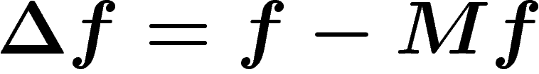$\Delta f=f-Mf$ . (Note that sometimes the renormalization by $1/\mathrm{deg}\,x$ is omitted in this definition.)

The averaging operator and the Laplacian are self-adjoint operators on the space $L^2(\Gamma,\mathrm{deg})$ of functions on $\Gamma$ (with the degree as a measure) and thus have a well-defined real spectrum. The spectrum of M is included in the interval $[-1;1]$ and always contains $1$ (take a constant function) and, thus, that of $\Delta$ lies in $[0;2]$ and always contains $0$ (with multiplicity $1$ when the graph is connected).

From now on we suppose that the graph is finite (so that we deal with true eigenvalues), connected (so that the eigenvalue $1$ is of multiplicity $1$ only), and of course without isolated points.

The spectral gap (often denoted $\lambda_1$ ) of the graph is the smallest non-zero eigenvalue of $\Delta$ , which is also the gap between $1$ and the largest non- $1$ eigenvalue of M.

The spectral radius of the graph has several definitions (depending on how negative eigenvalues [which corresponds to almost-bipartite graphs] are taken into account). The one we use is the following one: the spectral radius is the largest modulus of an eigenvalue of M distinct from $1$ . This is the quantity which is most relevant for the asymptotic speed of convergence of the simple random walk on $\Gamma$ . In particular, the spectral radius is not equal to $1$ minus the spectral gap. For example, for a bipartite graph, $-1$ is an eigenvalue of the averaging operator, and so the spectral radius is $1$ whereas the spectral gap is typically non-zero.

(Of course all these definitions can be adapted to the "symmetric Markov chain" setting when the edges bear different weights. This is not covered by our program.)

(Note on the treatment of loops in an unoriented graph: a loop is treated as both an ingoing and outgoing edge, so that it increases the degree by $2$ . The total number of edges is thus always half the sum of all degrees.)

Comments on the code and algorithm

The code was intended for use on very large, possibly very irregular graphs (typically random graphs), for which I did not want to diagonalize the adjacency matrix either symbolically or numerically.

So I decided to rely on a simple randomized algorithm to compute the second largest eigenvalue of a symmetric matrix: take a random centered gaussian vector and iterate the matrix on it a large number of times. Typically the initial vector has a non-zero component along the eigenvector associated to the second largest eigenvalue, and so eventually this component will become dominant.

Note that this easily provides a lower bound on the largest eigenvalue: indeed, taking any normalized vector, applying the matrix and computing the norm of the result gives such a bound. The difficult part is getting an upper bound.

So when the function SpecRad() of the program is invoked, two series of number are printed. Each line corresponds to one more iteration of the algorithm. The two numbers on each line are respectively a lower and upper bound for the spectral radius of the graph.

The lower bound is proved, i.e. if the program could handle arbitrary precision in number representation, it could output a proof.

However, the upper bound is probabilistic only. Let us insist that this probability is with respect to some random choice made by the program and not to some putative property of the graph or of mathematics. So whatever the graph is, in 95% of runs, the program prints a true mathematical statement, whereas it may be false in 5% in the runs. In particular, independent runs of the program on the same graph allow to reduce the failure probability (at least if the random number generator is sound.)

The probability of error is explicitly known and can be adjusted, see below.

For the spectral gap (function Lambda1()) the situation is reversed: the upper bound is proved, whereas the lower bound is probabilistic.

Use of the program

The sample file should be quite self-explanatory. After extracting the archive, modify the file example.cpp to provide the description of your favorite graph, then type make and run the specgraph file.

The variable specgraph_probaerror controls the probability of error allowed. specgraph_maxiter sets the maximal number of iterations before the search stops. specgraph_stopthreshold allows to stop the algorithm when a certain difference between the upper and lower bounds is reached. A call to randomize() is required to initialize the random number generator.

Construction of a graph is made by declaring a variable Graph, taking the number of vertices as an argument. Edges are added through the member function AddSymEdge(vertex number, vertex number). Vertices are numbered from $0$ to $n-1$ . A call to either member function Lambda1() or SpecRad() causes the program to print the bounds on screen.

The behavior of the program in unspecified in case the graph is not connected or has only one point.

Copying

This code is placed in the public domain. However, appropriate mention of credit is hoped for. Feedback about use of the program would be appreciated.

This sofware comes with absolutely no warranty.

Back to: Main Page > Mathematical programs

To leave a comment: contact (domain) yann-ollivier.org